Time Series Analysis is a statistical approach to studying and modeling data points collected sequentially over time. It’s used to understand patterns, trends, and behaviors in the data, and often to forecast future values based on those insights. Unlike random data sets, time series data has a natural temporal ordering—think stock prices, weather measurements, or website traffic logged hourly, daily, or monthly.
Core Components
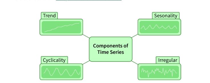
Time series data typically exhibits these elements:
- Trend: A long-term movement in the data, like a steady increase in global temperatures or a stock’s gradual rise.
- Seasonality: Repeating patterns tied to fixed intervals, such as higher retail sales every December or daily spikes in electricity use at 6 PM.
- Cyclic Patterns: Longer, less regular fluctuations, like economic booms and busts over years, not tied to a fixed calendar schedule.
- Noise: Random, unpredictable variations—like sudden market drops due to unexpected news—left after accounting for trend, seasonality, and cycles.
Main Goals
- Description: Identify and summarize patterns (e.g., “Sales peak every summer”).
- Explanation: Model relationships, like how past values or external factors (e.g., interest rates) influence the series.
- Forecasting: Predict future points, such as next quarter’s revenue or tomorrow’s weather.
- Control: Monitor and adjust processes, like tweaking a thermostat based on temperature trends.
Key Techniques
Descriptive Methods:
- Smoothing: Moving averages or exponential smoothing to reduce noise and highlight trends.
- Decomposition: Split the series into trend, seasonal, and residual components.
Stationarity Testing:
- Many models assume stationarity (constant mean and variance over time). Tests like the Augmented Dickey-Fuller (ADF) check this; if non-stationary, differencing or transformations (e.g., logarithms) can stabilize it.
Modeling:
- ARIMA (AutoRegressive Integrated Moving Average): Combines autoregression (past values predict future ones), differencing (to make data stationary), and moving averages (past errors inform predictions). Widely used for non-seasonal data.
- Seasonal ARIMA (SARIMA): Extends ARIMA to handle seasonality.
- Exponential Smoothing: Weights recent observations more heavily for forecasting, like Holt-Winters for trends and seasonality.
- Spectral Analysis: Uses tools like the Discrete Fourier Transform to identify dominant frequencies or cycles in the data.
Machine Learning:
- Techniques like LSTM (Long Short-Term Memory) neural networks or Prophet (from Meta) handle complex, non-linear patterns in big datasets.
Example
Suppose you’re analyzing daily stock prices:
- Trend: Prices rise over months due to company growth.
- Seasonality: Small dips every Monday as traders adjust positions.
- Noise: A sudden drop after a CEO scandal.
- Using ARIMA, you’d fit a model to past prices, then predict tomorrow’s value, adjusting for these patterns.
Applications
- Finance: Forecasting stock prices or volatility.
- Economics: Predicting GDP or unemployment rates.
- Meteorology: Modeling temperature or rainfall.
- Business: Inventory planning based on sales trends.
Time Series Analysis is powerful because it respects the sequential nature of data, letting you extract meaning from the past to anticipate the future. It blends stats, math, and domain knowledge to turn timestamps into insights.