What It Is
Bayes’ Theorem is a fundamental principle in probability theory that describes how to update the probability of a hypothesis based on new evidence. Named after the 18th-century mathematician Thomas Bayes, it provides a mathematical framework for reasoning under uncertainty, flipping the perspective from “what’s the chance of evidence given a hypothesis” to “what’s the chance of a hypothesis given the evidence.” It’s the backbone of Bayesian statistics, which treats probabilities as degrees of belief that evolve with data, unlike frequentist approaches that view probabilities as long-run frequencies. Bayes’ Theorem is widely used in fields like machine learning, medical diagnosis, spam filtering, and even everyday decision-making, offering a logical way to refine predictions as information accumulates.
At its core, Bayes’ Theorem connects prior knowledge (what you believe before seeing evidence) with new data (the evidence itself) to produce a revised belief (the posterior). It’s particularly powerful in situations where direct probabilities are hard to compute, but conditional relationships are known. Think of it as a tool for “learning from experience”—it quantifies how evidence shifts your confidence in a hypothesis, making it a cornerstone of probabilistic reasoning.
Key Takeaways
- Bayes’ Theorem allows you to update the predicted probabilities of an event by incorporating new information.
- Bayes’ Theorem was named after 18th-century mathematician Thomas Bayes.
- It is often employed in finance to calculate or update risk evaluation.
Formula
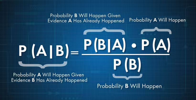
Bayes’ Theorem is expressed as:

Where:
- ( P(A|B) ): The posterior probability, the probability of hypothesis ( A ) given evidence ( B ).
- ( P(B|A) ): The likelihood, the probability of observing evidence ( B ) if hypothesis ( A ) is true.
- ( P(A) ): The prior probability, the initial probability of hypothesis ( A ) before seeing evidence ( B ).
- ( P(B) ): The marginal probability of the evidence ( B ), acting as a normalizing constant to ensure probabilities sum to 1.
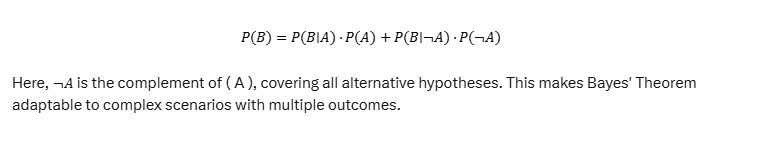
The denominator ( P(B) ) can be expanded using the law of total probability if ( A ) has multiple possible states (e.g., ( A ) and not-( A )):
Examples
Example 1: Medical Diagnosis
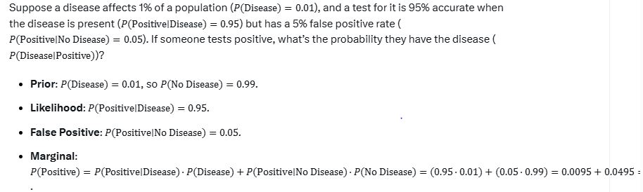
Now apply Bayes’ Theorem:

So, there’s only a 16.1% chance they have the disease, despite the positive test, because the disease is rare and false positives outweigh true positives in absolute terms. This highlights Bayes’ strength in adjusting for base rates.
Example 2: Weather Prediction
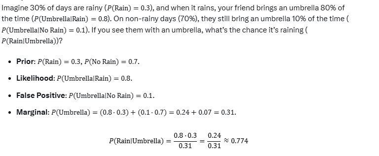
There’s a 77.4% chance it’s raining, showing how the umbrella strongly updates the prior belief.
Example 3: Spam Filtering
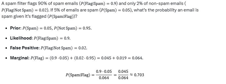
A flagged email has a 70.3% chance of being spam, refined by balancing the filter’s accuracy with spam rarity.
Why It Matters
Bayes’ Theorem excels at handling uncertainty, integrating prior knowledge with new data in a coherent way. It’s intuitive—evidence adjusts belief—and practical, powering tools like Bayesian networks and diagnostic systems. Its iterative nature (today’s posterior becomes tomorrow’s prior) mirrors how we learn, making it a timeless framework for understanding probability in an uncertain world.