A probability distribution is a mathematical description that shows how the possible values of a random variable are distributed according to their probabilities. It tells us which outcomes are more likely to occur and which are less likely, providing a structured way to represent uncertainty. Instead of predicting a single result, it describes all possible outcomes together with how frequently or how likely each one is expected to happen.
In general, probability distributions are used to model randomness in real-world situations. Many natural and human-made processes involve uncertainty, such as weather patterns, measurement errors, exam scores, or waiting times. By assigning probabilities to outcomes, a probability distribution helps researchers and analysts understand patterns hidden within random events and make informed predictions.
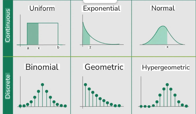
Probability distributions are usually grouped into two main categories: discrete and continuous. Discrete distributions apply when outcomes can be counted individually, such as the number of students in a class or the number of successful trials in an experiment. Continuous distributions apply when outcomes can take any value within a range, such as temperature, height, or time. Each type uses different mathematical tools but serves the same purpose of describing likelihood.
An important feature of any probability distribution is that all probabilities must follow specific rules. Every probability value must lie between zero and one, and the total probability of all possible outcomes must equal one. These rules ensure consistency and allow probabilities to represent real chances accurately. Graphs, tables, or formulas are commonly used to represent distributions visually or mathematically.
Probability distributions also allow calculation of key summary measures such as the mean, variance, and standard deviation. The mean represents the expected average outcome, while variance and standard deviation describe how spread out the values are around that average. These measures help compare datasets and understand whether results are tightly clustered or widely scattered.

Types of Probability Distribution
Normal Distribution
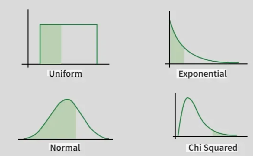
The normal distribution is a continuous probability distribution that forms a symmetrical, bell-shaped curve centered around the mean. Most values cluster near the average, while extreme values become increasingly rare as you move away from the center. It is widely used to model natural measurements and random processes.
Example: human heights in a large population often follow this pattern, where most people are close to the average height and very tall or very short individuals are less common.
Binomial Distribution
The binomial distribution describes the number of successes in a fixed number of independent trials where each trial has only two possible outcomes, such as success or failure. The probability of success remains constant across trials.
Example: counting how many times a coin lands on heads after flipping it 10 times can be modeled using this distribution.
Poisson Distribution
The Poisson distribution models how many times an event occurs within a fixed interval of time or space when events happen independently and at a constant average rate. It is useful for rare or random events.
Example: the number of customers arriving at a small shop per hour or the number of typing errors on a page.
Uniform Distribution
In a uniform distribution, all outcomes within a certain range have equal probability. There is no preference for any value over another within the interval. This distribution represents complete randomness within limits.
Example: selecting a random number between 1 and 10 where each number has the same chance of being chosen.
Exponential Distribution
The exponential distribution describes the time between events in a process where events occur continuously and independently at a constant average rate. It is often used in waiting-time problems.
Example: the amount of time a person waits before the next bus arrives when buses come randomly but at a steady average rate.
Geometric Distribution
The geometric distribution measures the number of trials needed to achieve the first success in repeated independent experiments with two outcomes. Unlike the binomial distribution, it focuses on when the first success happens.
Example: counting how many times a coin must be flipped before it lands on heads for the first time.
Beta Distribution
The beta distribution is a continuous distribution defined between 0 and 1, often used to model probabilities or proportions. Its shape can vary widely depending on its parameters, making it flexible for representing uncertainty about probabilities.
Example: estimating the probability that a student answers a question correctly after observing previous test results.
Gamma Distribution
The gamma distribution models the waiting time until multiple events occur in processes where events happen continuously and independently. It generalizes the exponential distribution by considering more than one event.
Example: measuring the total waiting time until three customers arrive at a service counter when arrivals happen randomly over time.
Bernoulli Distribution
The Bernoulli distribution is the simplest probability distribution and describes a single experiment with only two possible outcomes, usually called success and failure. Each outcome has a fixed probability, and only one trial is considered.
Example: checking whether a light bulb works or does not work when switched on can be modeled using this distribution.
Hypergeometric Distribution
The hypergeometric distribution models the probability of successes when sampling without replacement from a finite population. Because items are not returned after selection, probabilities change with each draw.
Example: selecting 5 cards from a deck and counting how many are hearts without putting any cards back.
Negative Binomial Distribution
The negative binomial distribution describes the number of trials required to achieve a specified number of successes in repeated independent experiments with constant success probability. It extends the geometric distribution to more than one success.
Example: determining how many basketball shots a player must attempt to make 4 successful shots.
Chi-Square Distribution
The chi-square distribution is a continuous distribution commonly used in statistical testing and data analysis, especially for testing relationships between categorical variables and measuring variability. It is always positive and depends on degrees of freedom.
Example: testing whether observed survey results differ significantly from expected results in a population study.
Student’s t-Distribution
The Student’s t-distribution is similar to the normal distribution but has heavier tails, making it useful when working with small sample sizes or unknown population variance. It is widely used in hypothesis testing and confidence intervals.
Example: estimating the average test score of a class using results from a small sample of students.
F-Distribution
The F-distribution is used mainly in comparing variances between two or more groups. It plays an important role in analysis of variance (ANOVA) and regression analysis. The distribution is skewed and depends on two sets of degrees of freedom.
Example: comparing the performance variability of students from different schools to see if their score differences are statistically significant.
Log-Normal Distribution
A log-normal distribution occurs when the logarithm of a variable follows a normal distribution. Values are positively skewed, meaning they cannot be negative and large values occur occasionally.
Example: modeling income levels or stock prices, where most values are moderate but a few are extremely large.
Weibull Distribution
The Weibull distribution is a flexible continuous distribution commonly used in reliability analysis and survival studies. It helps describe the lifespan of objects and failure rates over time.
Example: estimating how long machine parts or electronic components are likely to last before failing.
Cauchy Distribution
The Cauchy distribution is a continuous probability distribution with a bell-shaped curve similar to the normal distribution but with much heavier tails. Because of these extreme tails, its mean and variance are undefined, making it unusual in statistics.
Example: it can model measurement errors in certain physical experiments where extreme deviations occur more often than expected.
Rayleigh Distribution
The Rayleigh distribution is used to describe the magnitude of a vector whose components are independent and normally distributed. It commonly appears in signal processing and physics.
Example: modeling the strength of a wireless signal that varies due to random environmental effects.
Pareto Distribution
The Pareto distribution represents situations where a small number of occurrences account for a large portion of the effect, often called the “80–20 rule.” It is used in economics and social sciences to describe unequal distributions.
Example: a small percentage of people owning a large share of total wealth in a population.
Logistic Distribution
The logistic distribution resembles the normal distribution but has slightly heavier tails and is often used in growth models and logistic regression. It is helpful for modeling probabilities that change over time or conditions.
Example: predicting the probability that a student passes an exam based on study time.
Multinomial Distribution
The multinomial distribution generalizes the binomial distribution to experiments with more than two possible outcomes in each trial. It models counts across several categories simultaneously.
Example: rolling a six-sided die multiple times and counting how often each number appears.
Dirichlet Distribution
The Dirichlet distribution is a multivariable generalization of the beta distribution and is used to model probabilities that must add up to one. It is often applied in Bayesian statistics and machine learning.
Example: estimating the proportion of votes different candidates may receive before an election.
Laplace Distribution
The Laplace distribution, sometimes called the double exponential distribution, has a sharp peak at the mean and heavier tails than the normal distribution. It is useful for modeling data with frequent small changes and occasional large deviations.
Example: representing differences between predicted and actual values in certain economic or engineering models.
Power Law Distribution
The power law distribution describes phenomena where large events are rare but extremely influential, and small events are very common. It appears in many natural and social systems.
Example: modeling earthquake magnitudes, where small tremors occur often but very large earthquakes are rare yet impactful.
Wishart Distribution
The Wishart distribution is a probability distribution defined over positive-definite matrices and is often considered a multivariate extension of the chi-square distribution. It is mainly used in multivariate statistics to model sample covariance matrices. This distribution plays an important role in statistical inference involving multiple correlated variables.
Example: estimating the covariance matrix of several exam subjects (such as math, science, and language scores) collected from many students.
Multivariate Normal Distribution
The multivariate normal distribution generalizes the normal distribution to multiple variables that may be correlated with each other. Instead of a single mean and variance, it uses a mean vector and a covariance matrix to describe relationships between variables. It is widely used in machine learning, finance, and scientific modeling.
Example: modeling height and weight together in a population, where both measurements vary normally but are also related.
Quadratic Form Distribution
A quadratic form distribution arises when a quadratic expression involving random variables is studied, typically written as a vector multiplied by a matrix and then by the vector again. These distributions appear frequently in statistical testing and estimation theory, especially when analyzing variance and energy-like quantities.
Example: calculating sums of squared deviations in regression analysis or hypothesis testing, where squared combinations of variables determine test statistics.
Evolving (Time-Dependent) Distributions
An evolving probability distribution refers to a distribution that changes over time according to some stochastic or dynamic process rather than remaining fixed. Such distributions are studied in stochastic processes, filtering theory, and dynamical systems.
Example: modeling how stock price probabilities change daily as new market information arrives, or how the distribution of particles spreads out over time in diffusion processes.